Images of metabolic rate of oxygen in the brain using [15O]O2-PET
Single inhalation [15O]O2 bolus model
The metabolic rate of oxygen in the brain has been measured with steady-state and bolus inhalation techniques (Herscovitch 1995). Radiation dose to the patient is smaller in the single bolus inhalation than in the "gold standard" steady-state techniques, because separate [15O]H2O and [15O]CO studies are not needed. Single inhalation bolus also require less scanner time. Techniques that require several PET scans may be unreliable if subject can move between the scans (Correia et al. 1985).
Bolus inhalation models are based on the study of Mintun et al. (1984), in
which perfusion and blood volume were still measured in separate PET studies.
In this two-compartment model it is assumed that blood flow f delivers
a certain amount of labeled oxygen into the blood volume in the tissue. A
fraction of this oxygen (OEF, oxygen extraction fraction) is diffused
to tissue and metabolized instantly to labeled water; the remaining fraction
of delivered oxygen (1-OEF) is flushed from the tissue with blood
flow. Labeled water is flushed away from the tissue with rate constant
f/p, where p is the partition constant of the water. During the
PET scan, labeled water is also formed elsewhere in the body, and it is
delivered to brain from arterial blood with perfusion f and washed
away like the labeled water that is formed in the brain. If the oxygen
concentration in arterial blood, [O2]a, is measured,
then the metabolic rate of oxygen (MRO2) can be calculated
as:
Notice that equation for calculating [O2]a may be different in animals than in humans (Poulsen et al., 1997).
It is not necessary to measure the blood flow or blood volume separately, because f*OEF and VB can be estimated from a single inhalation [15O]O2 study (Holden et al. 1988).
Ohta et al. (1992) have further simplified the calculation model. This model can be linearized (Blomqvist 1984; Poulsen et al., 1997), which permits the pixel-by-pixel computation. Unlike for the previous models, in this method the separation of [15O]O2 and [15O]H2O in arterial blood is not necessary. When the duration of the study (time that is used in the model fit) is limited to 3 minutes, and the oxygen consumption is in the range 50-300 μmol/(min 100 g), the error caused by ignoring the recirculating radiowater will remain between ±10% (Ohta et al. 1992).
Performance of the model can be studied with simulations, for an example see the study by Duval et al. (2002).
Steps of MRO2 calculation:
1. Pre-processing of arterial blood curve
Arterial blood data from the on-line sampler needs to be processed before it can be used as input function in the calculation.
If you are working in TPC, use the script water_input to process the on-line detector (blood pump) data prior to the analysis. It requires the countrate curve (*.cr) or similar data for the time delay correction; time delay correction is necessary in order to obtain non-biased oxygen consumption estimates (Poulsen et al., 2007). Notice that in [15O]O2 PET studies the countrate curve has often been unusable, probably because of high random counts from dose collection system and/or exhaling of 15O gases; then we would advice to create "head curves" from dynamic PET images using ecathead for all studies and use these instead of countrate curves.
The corrected blood TAC should always be plotted and controlled visually. Water_input script creates a post-script (.ps) format plot of corrected input curve and countrate curve. Corrected blood curve often contains close-to-zero values in the end, which should be removed with a text editor, or left out when determining the fit time. Check also that sample times are in seconds, not minutes.
2. Compute K1 image
Before calculation
- make sure that both the blood and PET image are in the same calibration units (preferably kBq/ml); image data from HR+ and PET-CT may originally be in units Bq/ml, while blood data are in units kBq/ml.
- if necessary, reduce the noise in dynamic PET image.
- if necessary, correct the dynamic image for the contribution of vascular radioactivity using a measured or population average based VB. Because of high noise-level of pixels, fitting VB as one model parameter is not recommended.
Calculation of K1 image
Compute the K1 (=f*OEF) image using imgflow with the following command-line arguments:
- option
-Va=noneto prevent an additional VB correction, if vascular volume was previously corrected - corrected arterial blood datafile that was made in step one (times in seconds)
- VB-corrected dynamic [15O]O2 image file
- fit time in seconds (max 180 in this model)
- filename for the K1 image
The units in the [15O]O2 image are (mL blood)/(min * mL tissue) by default.
3. Conversion of K1 image to MRO2 image
The metabolic rate of oxygen is calculated by multiplying the
K1 (=f*OEF) image by the concentration of
O2 in arterial blood:
MRO2 = K1*[O2]a.
Program ecatcalc can be
used for this purpose.
Turku PET Centre gets the arterial oxygen concentrations from the hospital laboratory in units ml O2/L blood, which must be converted to mL O2/100 mL blood; the oxygen concentrations are normally about 20 mL O2/100 mL blood (100 mL = 1 dL). If MRO2 is required in molar units, then [O2]a must be divided by the molar volume of an ideal gas, 22.4 mL/mmol; thereafter [O2]a values are about 0.9 mmol O2/100 mL blood.
After the multiplication, the unit of the MRO2 image is either mL O2 / (min * 100 mL tissue) or mmol O2 / (min * 100 mL tissue), depending on the unit of [O2]a. If MRO2 is required per tissue mass instead of volume, the image can be divided by tissue density (specific gravity), 1.04 g/mL (Reference Man).
Cerebral MRO2 in normal subjects are in the range of 2.2 to 3.5 mL O2 / (min * 100 g tissue) in gray matter (Perlmutter et al. 1987; Leenders et al. 1990).
The MRO2 image can then be used in SPM analysis, and/or ROIs can be drawn and regional MRO2 values calculated using e.g. img2dft.
Example of MRO2 image
Below are two MRO2 images calculated from the same PET study,
where dynamic image was reconstructed with FBP and normal parameter settings.
In the latter case, dynamic image was further
filtered
before calculation of K1 image using
imgdysmo
with options -m=5 -s=4.
Images are not in the same color scale.
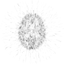
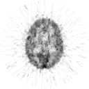
The results from parametric images should always be checked against results from regional curves. Noise in dynamic image may lead into biased results with distorted variance. Filtering of dynamic images may be needed to achieve the same quantitative results as in the regional analysis. To prevent artefacts and excessive loss of image resolution, the strength of filtering must not exceed the level that is required to achieve comparable results.
See also:
- Pre-processing of arterial on-line blood sampler data
- Regional metabolic rate of oxygen in the brain
